
Background
The purpose of a business has always been to serve the demand of its customers at expected quantity, expected price and expected quality. These expectations create the need to estimate what is the right quantity, price as well as quality of the product in order for it to make sense for targeted customers.
Introduction
In this post, I would like to focus the rest of the discussion around quantity estimation or in other words demand estimation.
Estimating or predicting future has always been a difficult task & the problem becomes even more complicated when you need to estimate the demand at lower levels. The difficulty of the problem increases exponentially as we move from company level to business unit level to product family level to SKU level. Estimating demand at higher levels yields us leading indicators for better business planning. However, at actual manufacturing and retail store level we are often required to estimate demand for each SKU in order to utilize our resources in the best possible way & to keep a tab on ever increasing inventory levels while maintaining a fine balance with customer service level.
Approach
I would like to divide the approach to tackle this problem under two broad level categories:
1) Time Series Forecasting
2) Machine Learning Forecasting
Time Series Forecasting
By time series, I am referring to the traditional way of estimating the future of a variable, which in this case is demand, using the historical data of same variable. So, we try to extract any hidden trend or pattern in the historical demand of the product & extrapolate that pattern to predict future demand. Now the most common technique that we usually resort to in such scenarios is ARIMA. I am not going into the details of ARIMA methodology here but the one methodology that we usually come across during our academic courses or studies involve estimating ARIMA parameters — p,d,q (or in some cases their seasonal counter parts as well) by carrying out stationarity tests & then visually inspecting auto-correlation or partial auto-correlation plots to arrive at appropriate estimates for ARIMA parameters. Though this technique provides us greater understanding of the inherent time series structure, it poses a challenge when the same exercise needs to be repeated at a larger scale, say for tens of thousands of time series.
Again, this method can be further divided into two streams:
a) Without exogenous variables
In case demand of the product at various historic timestamps is the only information available, we should try out different families of time series methodologies like ETS, ARIMA, TBATS, etc. & pick the one that gives the minimum error or information loss in the validation set. Rather than taking our decision based on one validation set, we try out a cross validation approach & then select the approach that has minimum cross validation error. Only thing to keep in mind in such scenarios is the peculiarity nature of time series data. Unlike the traditional machine learning approach where we would divide the dataset arbitrarily (or do a stratified sampling), each cross validation set derived from a time series data needs to be taken from a contiguous block of timestamps as the pattern or relationship is generally estimated based on the relative time lag position of historical readings.
b) Without exogenous variables
In some cases, apart from the historical demand data for each SKU, we also have some other independent data points like forecast from sales team, forecast from customer, industry or segment demand numbers, promotional plans, etc. To utilize these factors while generating the forecast numbers, we can include these external parameters in the model as well. Such techniques are known by the names of ARIMAX or Dynamic Regression (as Rob Hyndman suggests). The idea is that we first apply a time series technique like ARIMA using the historical data & the remaining error terms from this exercise are further regressed against the available external variables. The underlying concept relies on explaining maximum variation in the data using both time series & linear regression. Appropriate technique for each SKU could then be selected again by using cross validation error.
However, if you are implementing this in R using forecast package, you might have to write your own function for cross validation part as default functions may not directly support cross validation using dynamic regression.
Machine Learning Forecasting
The machine learning approach can also be divided under two heads:
A) Without clustering
The idea here is to arrange the data available at each SKU level & convert it from a univariate data structure to a multivariate structure of inputs.
a) Without exogenous variables
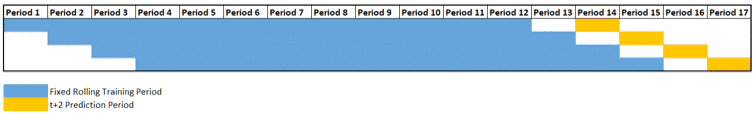
When external variables are not available, we can convert data available at different lags into input feature set. Demand value present at prediction time step becomes the target variable in such scenarios.
![]()
The initial lag value, N, is to be considered based on the understanding of business & we can also try out a set of N values & use grid search to evaluate the number of lags to be considered while building the model. Prediction time step h will again vary from business to business & we generally try to keep the value of h in such a way that would leave enough time for the rest of the supply chain to react to the change in demand, if any. Arranging the data in such a columnar structure allows to use even tree-based machine learning algorithms & we are no longer restricted to the linear relationships. Time series models in a way look at only the linear relationship with respect to various lags & hence significantly different results could be obtained using different non-parametric machine learning models in this case.
b) With exogenous variables
In case where external market signals or other internal demand signals are present at SKU level then these could also be incorporated into the machine learning model.
This approach would differ greatly from the approaches that have been mentioned so far in this post as in this case we would avoid building individual models for each of the SKUs. We would rather try to understand the historic demand pattern of all the SKUs & then try to group together those which follow similar demand pattern. We can either use the actual demand numbers or opt to generate summary statistics of historical demand numbers to segregate the SKUs with similar demand distribution.
Once we are able to identify right segments or clusters of SKUs, the next step would involve building individually optimized models for each of those segments.
This approach helps us two folds — First, it reduces the complexity of developing and managing so many individual models; Second, we would now have enough data to actually tune the model parameters & in case the data points in each cluster are sufficient, we may even try out neural networks (in case you fancy that)
Again, inclusion of external variables would vary from case to case depending upon whether relevant external variables are available in your industry or not.
When I initially started working in this area, I had to spend a lot of time in formulating the right approach where demand forecasting needs to be carried out at scale. Hope this post gives you a head start in case you plan to work on similar problem.
P.S. I have not touched upon the data sparsity related issues here which would call for careful analysis of data while building the models at granular level. You may like to understand how parameters like coefficient of variation (CoV) can help you first assess the forecastability of the concerned SKUs or categories, even before proceeding with the model development exercise.